Tree-based Machine Learning Models 트리 기반 모델 1
Decision tree, Bagging, Random forest, Boostring등 현재 업계에서 많이 사용되는 트리 기반 모델에 대해 알아본다.
1. 트리기반 모델이란?
트리기반 의사 결정 모델은 feature space를 여러 개의 영역으로 나누는 것을 목표로 동작하는 알고리즘이다.
feature space를 평균(회귀) 또는 모드(분류)를 기반으로 주어진 관찰에 대한 예측을 수행한다.
2. 트리 기반 모델의 평가 척도
트리기반 의사 결정 모델은 Impurity(불순도)로 측정되며 설정된 불순도 기준에 따라 변수가 Stopping criteria(중지 기준)에 도달할 때까지 반복적으로 분할한다.
불순도 측정 척도는 크게 세 가지가 이용된다.
1) Entropy 엔트로피
샘플이 완전 균질하면 엔트로피는 0, 샘플이 마구 섞여 있으면 엔트로피가 1로
엔트로피는 중간에서 최대값을 가지며 그 값은 1이고 극값은 0으로 최소값을 가진다.
즉, 데이터가 서로 다른 종류끼리 섞여있으면 엔트로피가 높고 비슷한 종류끼리 섞여있으면 엔트로피가 낮다.

2) Information Gain 정보 획득
의사결정트리에서 정보 획득은 고유 정보에 대한 정보 획득 비율이다.
즉, 어떤 변수를 선택하냐에 따라 데이터를 잘 구분할 수 있는지를 나타내는 척도이다.

information gain = 상위 엔트로피 - (가중치 % x 하위 엔트로피)의 합계
3) Gini 지니
오분류의 척도로 엔트로피와 유사하게 작동하지만 Gini 계산법이 더 빠르다.
gini impurity = 0 이면 집단은 완벽하게 순수하다(pure)는 뜻이다.
다시 말해, 비슷한 집단끼리 잘 분류되어 있다는 것을 의미한다.


3. 트리분류모델 작동 방법
테니스 경기 여부 예제(whether to play tennis or not)


데이터 셋에서 Humidity와 Wind 중 어떤 변수가 테니스 경기에 더 영향을 끼치는 지 알아보도록 한다.
1) Humidity 변수
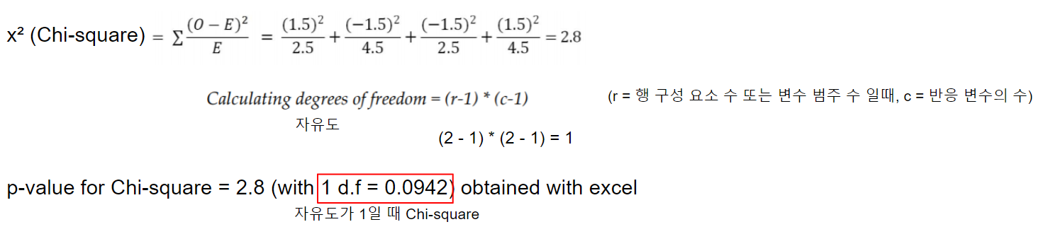
- CHAID(Chi-Squared Automatic Interaction Detection)
: 카이 제곱 검정(이산형 목표 변수) 또는 F-검정(연속형 목표 변수)을 이용해 다자분리를 수행하는 알고리즘
- Entropy, Information Gain


- Gini


2) Wind 변수
- CHAID(Chi-Squared Automatic Interaction Detection)

- Entropy, Information Gain

- GINI

두 변수의 세 가지 검사 결과 비교표는 다음과 같다.

CHAID의 경우 값이 낮을수록 좋고,
Entropy, Information gain은 값이 높을수록 좋으며
Gini expected value는 값이 낮을수록 좋다.
따라서 두 변수 중 테니스 경기에 더 영향을 미치는 변수는 Humidity인 것을 알 수 있다.
4. 로지스틱 회귀와 의사결정트리 비교
| Logistic regression | Decision trees |
| 종속 변수와 독립 변수 간의 방정식처럼 보임 | 간단한 영어분장으로 규칙 생성 가능 |
| 매개 변수를 독립 변수로 곱하여 종속 변수를 예측하여 모델을 정의하는 매개 변수 모델 | 미리 가정된 매개 변수가 없는 비모수 모델 |
| 이상 또는 베르누이 분포를 사용하여 반응(또는 종속) 변수에 대해 가정 | 데이터의 기본 분포에 대한 가정 없음 |
| 모델의 모양이 미리 정의되어 있음 (로지스틱 곡선) | 모델의 모양은 미리 정의되어 있지 않음 대신 데이터를 기반으로 최상의 분류에 적합함 |
| 독립 변수가 본질적으로 연속적이고 선형성이 참일 때 매우 좋은 결과를 제공 | 대부분의 변수가 범주형일 때 최상의 결과를 제공 |
| 변수 간의 복잡한 상호작용을 찾기 어려움 (비선형 변수 같의 관계) |
매개 변수 간의 비선형 관계는 트리 성능에 영향을 주지 않고 종종 복잡한 상호작용을 발견함 고도로 치우치거나 다중 모드로 숫자 데이터를 처리할 수 있을 뿐만 아니라 순서형 또는 비순서형 구조를 사용하는 범주형 예측 변수를 처리할 수 있음 |
| 특이치와 결측치는 로지스틱 회귀에 성능을 저하시킴 | 특이치와 결측치는 의사결정트리에서 처리 가능함 |
5. 트리결정모델의 성능평가
트리모델의 성능 향상을 위해 모델의 오차를 평가할 수 있어야 한다.
오차 성분은 bias component(편향 성분), variance component(분산 성분), pure with noise(노이즈)로 구성되어 있다.

5-1. 모델 별 오차 구성의 비교

첫 번째 지역(주황색): 높은 bias와 낮은 variance -> linear or logistic regression model
두 번째 지역(녹색): bias와 variance 모두 중간 정도 -> ideal model
세 번째 지역(보라색): 높은 variance와 낮은 bias -> decision tree based model
-> linear 모델이나 decision tree 모델 모두 가운데 이상적인 지역에 속하도록 모델을 업그레이드 시켜야 한다.
5-2. 오차를 줄이기 위한 방법 비교

Linear model: high bias를 줄이기 위해 단일 선을 작은 선형 조각으로 나누어 선형 스플라인(주어진 데이터의 각 구간마다 추정함수를 구하는 것)이라고 하는 매듭 점으로 제한하여 영역에 맞춰 해결한다.
Decision tree model: high variance를 줄이기 위해 의사 결정 트리의 앙상블(여러 개의 분류기를 결합하여 하나의 분류기를 만드는 것)을 수행하여 해결한다.
6. 트리 모델 예제
kaggle의 IBM HR Analytics Employee Attrition & Performance 데이터를 이용하여
어떤 변수가 직원의 이직률에 큰 영향을 미치는지 알아보는 분석을 해본다.
1) Data 전처리
- 모듈 및 데이터 임포트
import pandas as pd

hrattr_data = pd.read_csv('./data/WA_Fn_UseC_-HT-Employee-Attrition.csv')

hrattr_data.head()
- Attrition 컬럼의 Yes 값을 1로 No 값을 0으로 바꿔 새로운 칼럼 Attrition_ind에 추가
hrattr_data['Attrition_ind'] = 0
hrattr_data.loc[hrattr_data['Attrition'] == 'Yes', 'Attrition_ind'] = 1

hrattr_data.head()
- 범주형 데이터를 컬럼 별로 dummy data 만들기 (one-hot encoding)
dummy_busnstrvl = pd.get_dummies(hrattr_data['BusinessTravel'], prefix='busns_trvl')
dummy_dept = pd.get_dummies(hrattr_data['Department'], prefix='busns_dept')
dummy_edufield = pd.get_dummies(hrattr_data['EducationField'], prefix='edufield')
dummy_gender = pd.get_dummies(hrattr_data['Gender'], prefix='gender')
dummy_jobrole = pd.get_dummies(hrattr_data['jobRole'], prefix='jobrole')
dummy_maritstat = pd.get_dummies(hrattr_data['MaritalStatus'], prefix='maritstat')
dummy_overtime = pd.get_dummies(hrattr_data['OverTime'], prefix='overtime')
- 연속형 변수로 구성된 컬럼과 dummy data로 만든 범주형 데이터와 합쳐주어 새로운 데이터 프레임 생성
continuous_columns = ['Age', 'DailyRate', 'DistanceFromHome', 'Education',
	'EnvironmentSatisfaction', 'HourlyRate', 'JobInvolvement', 'JobLevel',
    'JobLevel', 'JobSatisfaction', 'MonthlyIncome', 'NumCompaniesWorked',
    'PercentSalaryHike', 'PerformanceRating', 'RelationshipSatisfaction',
    'StockOptionLevel', 'TotalWorkingYears', 'TrainingLastYear', 'WorkLifeBalance',
    'YearAtCompany', 'YearsInCurrentRole', 'YearsSinceLastPromotion', 'YearsWithCurrManager']

hrattr_continuous = hrattr_data[continuous_columns]

hrattr_data_new = pd.concat([dummy_busnstrvl, dummy_dept, dummy_edufield,
	dummy_gender, dummy_jobrole, dummy_maritstat, dummy_overtime, hrattr_continuous,
    hrattr_data['Attrition_ind']], axis=1)
- 트레인, 테스트 셋으로 데이터 프레임 나눠주기
from sklearn.model_selection import train_test_split

x_train, x_test, y_train, y_test = train_test_split(hrattr_data_new.drop(['Arrrition_ind'], axis=1),
			hrattr_data_new['Attrition_ind'], train_size=0.7, random_state=42)
- Decision Tree Classifier 모델 생성 후 학습
from sklearn.tree import DecisionTreeClassifier

df_fit = DecisionTreeClassifier(criterion='gini', max_depth=5, min_samples_split=2,
			min_sample_leaf=1, random_state=42)

df_fit.fit(x_train, y_train)
- Decision Tree Classifier 모델 학습 후 confusion matrix, accuracy, precision, recall 값 확인
print("Decision Tree - Train Confusion Matrix\n")
pd.crosstab(y_train, df_fit.predict(x_train), rownames=["Actuall"], colnames=["Predicted"])

from sklearn.metrics import accuracy_score, classification_report

print("Decision Tree - Train accuracy\n", round(accuracy_score(y_train, df_fit.predict(x_train)), 3))

print("\nDecision Tree - Train Classification Report\n", classification_report(y_train, df_fit.predict(x_train)))

print("\nDecision Tree - Test confusion matrix\n", pd.crosstab(y_test, df_fit.predict(x_test),
			rownames=["Actuall"], colnames=["Predicted"]))

print("\nDecision Tree - Test accuracy", round(accuracy_score(y_test, df_fit.predict(x_test)), 3))

print("\nDecision Tree - Test Classification Report\n", classification_report(y_test, df_fit.predict(x_test)))
Test accuracy가 0.846으로 높은 편이지만, precision과 recall 값이 0.39와 0.20으로 매우 낮은 편이다.
-> Tuning이 필요하다.
- 튜닝할 하이퍼파라미터 설정
import numpy as np

dummyarray = np.empty((6, 10))

dt_wttune = pd.DataFrame(dummyarray)
dt_wttune.columns = ['zero_wght', 'one_wght', 'tr_accuracy', 'tst_accuracy', 'prec_zero',
		'prec_one', 'prec_ovll', 'recl_zero', 'recl_one', 'recl_ovll']

zero_clwghts = [0.01, 0.1, 0.2, 0.3, 0.4, 0.5]

for i in range(len(zero_clwghts)):
	clwght = {0:zero_clwght[i], 1:1.0-zero_clwght[i]}
    dt_fit = DecisionTreeClassifier(criterion='gini', max_depth=5, min_samples_split=2,
    		min_samples_leaf=1, random_state=42)
    dt_fit.fit(x_train, y_train)
    dt_wttune.loc[i, 'zero_wght'] = clwght[0]
    dt_wttune.loc[i, 'one_wght'] = clwght[1]
    dt_wttune.loc[i, 'tr_accuracy']= round(accuracy_score(y_train, dt_fit.predict(x_train)), 3)
    dt_wttune.loc[i, 'tst_accuracy']= round(accuracy_score(y_test, dt_fit.predict(x_test)), 3)
    clf_sp = classification_report(y_test, dt_fit.predict(x_test)).split()
    dt_wttune.loc[i, 'prec_zero'] = float(clf_sp[5)
    dt_wttune.loc[i, 'prec_one'] = float(clf_sp[10])
    dt_wttune.loc[i, 'prec_ovll'] = float(clf_sp[17])
    dt_wttune.loc[i, 'recl_zero'] = float(clf_sp[6])
    dt_wttune.loc[i, 'recl_one'] = float(clf_sp[11])
    dt_wttune.loc[i, 'recl_ovll'] = float(clf_sp[18])

print("\nClass Weight", clwght,
	"Train accuracy: ", round(accuracy_score(y_train, dt_fit.predict(x_train)), 3),
    "Test accuracy: ", round(accuracy_score(y_test, df_tif.precict(x_test)), 3)

print("\nTest confusion matrix", pd.crosstab(y_test, df_fit.predict(x_test),
	rownames=["Actuall"], colnames=["Predicted"]))
zero: 0.3, one: 0.7 일 때, 가장 높은 atrriers를 예측했다. (test accuracy: 0.839)
다음 편에서는 트리 기반 모델의 앙상블인 Bagging, Random forest, AdaBoost 등을 살펴보려 한다.
[참고문헌]
1. Pratap Dangeti, 2017, Statistics for Machine Learning