통계학의 선형회귀분석과 머신러닝의 Ridge, Lasso 회귀 모델 비교
1. 통계학 모델링과 머신러닝 모델링의 주요 차이점
| Statistics modeling | Machine learning |
| 방정식 형태로 변수 간의 관계를 공식화함 | 규칙 기반이 아닌 데이터에서 학습할 수 있는 알고리즘 |
| 데이터에 대한 모델 피팅 수행 전에 모델 곡선의 모양을 가정해야함 | 제공된 데이터를 기반으로 복잡한 패턴을 자동으로 학습할 수 있으므로 기본 형태를 가정할 필요 없음 |
| 85%의 정확도와 95%의 신뢰도로 output을 예측함 | 85%의 정확도로 output을 예측함 |
| 모델링에서 P 값과 같은 다양한 매개변수 진단이 수행됨 | 통계적 진단 테스트를 수행하지 않음 |
| 데이터는 train, test를 수행하기 위해 70-30%로 분할됨 학습 데이터에서 개발되고 테스트데이터에서 테스트된 모델 |
데이터는 train, validation, test를 수행하기 위해 50-25-25%로 분할됨 train 및 hyperparameter를 기반으로 개발된 모델은 validation 데이터라고 하는 두 개의 데이터 셋에서 기계학습 알고리즘을 훈련해야 함 |
| 전체 정확도와 개별 변수 수준에서 진단이 수행되므로 train 데이터는 단일 데이터 셋에서 통계 모델을 develop할 수 있음 | 변수에 대한 진단이 부족하기 때문에 two-point validation을 보장하려면 train 및 validation 데이터라고 하는 두 개의 데이터 셋에서 기계학습 알고리즘을 훈련해야 함 |
| 주로 연구 목적으로 사용 | 프로덕션 환경에서 구현하기 적합 |
| 통계학과, 수학과 | 컴퓨터공학과 |
Statistical Model
1. Adjusted R-squred 값을 이용해 훈련 데이터 검증에 대한 전체 모델 정확도
2. 훈련 데이터에 대한 개별 독립 변수 진단 검사
a. P값을 이용한 유의성 검사
b. VIF를 이용한 다중공선성 검사
Machine Learning Model
1. 훈련 데이터 평균 제곱 오차에 대한 전체 모델 정확도
2. hyperparameter를 조정하여 검증 데이터셋에 대한 전반적인 정확도를 가장 잘 파악함
학습 및 검증 데이터 모두에 가장 적합하다고 가정하여 모델이 보이지 않는 데이터에 대해 잘 일반화됨
2. 선형 모델의 가정
선형 모델은 다음의 가정을 따라야 한다.
1) 종속 변수는 독립 변수의 선형조합이어야 한다.
2) 오차항에서 자기상관이 없다.
3) 오차는 평균의 0이고 정규분포를 따라야 한다.
4) 다중공선성이 없거나 거의 없어야 한다.
5) 오차항은 공분산이어야 한다.
1) 종속 변수는 독립 변수의 선형조합이어야 한다.
y는 x 변수의 선형조합이어야 한다.
진단 방법: residuals vs fitted (잔차 대 독립변수)의 residuals 그래프를 관찰 또는 다항식 항을 포함하고 잔차 값의 감소를 확인
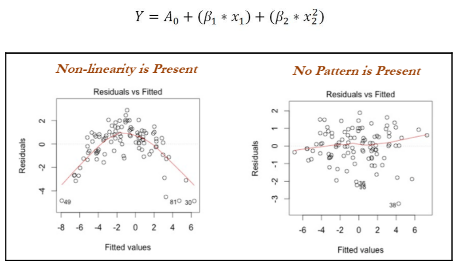
왼쪽 그래프의 경우 회귀가 적용되어 패턴이 있는 것처럼 보이나 검정력을 높인 후에는 오른쪽 그래프와 같이 패턴없는 nose로 나타나는 것을 알 수 있음
2) 오차항에서 자기상관(autocorrelation)이 없다.
오차항에서 상관관계가 있으면 모델 정확도가 떨어진다.
Durbin-Watson 검사를 통해 d는 잔차가 선형적으로 자기상관관계가 없다는 귀무가설을 검정한다.
* Durbin-Watson 검사: 회귀 모형의 오차에 자기 상관이 있는지 검정하는 검사로 자기 상관은 인접 관측치의 오차가 상관되어 있음을 의미하므로 오차가 상관되면 최소 제곱법이 계수의 표준 오류를 과소추정할 수 있음
3) 오차는 평균이 0이고 정규분포를 따라야 한다.
모델이 편향되지 않은 추정치를 생성하려면 오차의 평균이 0이어야 한다.
오차를 플로팅하면 오차 분포가 표시되는 반면 오차항이 정규분포를 따르지 않으면 신뢰구간이 너무 넓거나 좁아져 최소 제곱 최소화를 기반으로 계수를 추정하는데 어려움이 있음을 의미한다.
4) 다중공선성(Multicollinearity)이 없거나 거의 없어야 한다.

다중공선성은 독립 변수가 서로 상관관계가 있는 경우이며 이러한 상황은 계수 / 추정의 크기를 부풀려 불안정한 모델을 생성한다.
진단방법: 산점도를 살펴보고 데이터의 모든 변수에 대해 상관 계수를 실행분산 팽창 계수(VIF)를 계산
VIF <= 4 면 다중공선성이 없다고 보고 더욱 엄격한 환경(ex.은행)에서는 VIF<=2도 사용
5) 오차항은 공분산이어야 한다.

오차는 독립 변수들 간에 일정한 분산을 가져야 한다.
이로 인해 추정치에 대한 신뢰 구간이 비현실적으로 넓거나 좁아져 모델의 성능이 저하될 수 있다.
동분산성을 유지하는 않는 이유는 데이터에 특이치가 존재하기 때문이며 이로 인해 모델이 더 높은 가중치를 가진 이들에게 적합하다.
진단방법: residuals vs fitted 그래프를 관찰한다.
원뿔 또는 발산 패턴이 존재하는 경우 오류에 일정한 분산이 업서으므로 예측에 영향을 미친다.
3. 선형 회귀 모델링의 산업적 적용
다음 단계는 산업의 선형회귀 모델링에 적용된다.
1) 결측값 및 이상치 처리
2) 독립 변수의 상관관계 확인
3) 무작위 분류 학습 및 테스트
4) 학습 데이터에 모델 맞추기
5) 테스트 데이터에 대한 모델 평가
4. 선형 회귀 모델 예제
Example of simple linear regression using the wine quality data
1) 모듈 임포트 및 데이터 불러오기
import pandas as pd
from sklearn.model_selection import train_test_split
from sklearn.metrics import r2_score

wine_quality = pd.read_csv('winequality-red.scv', sep=';')
wine_quality.rename(colunms=lambda x: x.replace(" ", "_"), inplace=True)
2) 데이터 헤드값 확인하기
wine_quality.head()
3) 데이터를 훈련 및 테스트 셋으로 나눈 뒤, 평균, 절편, 상관계수를 구하기
x_train = pd.DataFrame(x_train); x_test = pd.DataFrame(x_test)
y_train = pd.DataFrame(y_trian); y_test = pd.DataFrame(y_test)

def mean(values):
    return round(sum(values) / float(len(values)), 2)

alcohol_mean = mean(x_train['alcohol'])
quality_mean = mean(y_train['quality'])

alcohol_variance = round(sum((x_train['alcohol'] - alcohol_mean) ** 2), 2)
quality_variance = round(sum((y_train['quality'] - quality_mean) ** 2), 2)

covariance = round(sum((x_train['alcohol'] - alhochol_mean) * (y_train['quality'] - quality_mean)), 2)

b1 = covariance / alcohol_variance
b0 = quailty_mean - b1 * alcohol_mean

print("Intercept (B0):", round(b0, 4), "Co-efficient (B1):", round(b1, 4))
Intercept(B0, 절편): 1.6918 / Co-effcient(B1, 상관계수): 0.377
4) 생성된 모델을 이용해 test 셋의 R-squared 값을 구하기
y_test['y_pred'] = pd.DataFrame(b0 + b1 * x_test['alcohol'])

R_sqrd = 1 - (sum((y_test['quality'] - y_test['y_pred']) ** 2) / sum((y_test['quality'])) ** 2))

print("Test R-squared value:", round(R_sqrd, 4))
Example of multilinear regression step-by-step methodology of model building
1) 모듈 임포트 및 데이터 불러오기
import numpy as np
import pandas as pd
import statsmodels.api as sm
import matplotlib.pyplot as plt
import seaborn as sns
from sklearn.model_selection import train_test_split
from sklearn.metrics import r2_score

wine_quality = pd.read_csv("winequality-res.csv", sep=';')
wine_quality.rename(columns=lambda x: x.replace(" ", "_"), inplace=True)

eda_colnms = ["volatile_acidity", "chlorides", "sulphates", "alcohol", "quality"]
sns.set(style="whitegrid", context="notebook")
2) 각 변수간 공분산을 그래프로 그리기 - 1
sns.pairplot(wine_quality[eda_colnms], size=2.5, v_vars=eda_colnms, y_vars=eda_colnms)
3) 각 변수간 공분산을 그래프로 그리기 - 2
corr_mat = np.corrcoef(wine_quality[eda_colnms].values.T)

sns.set(font_scale=1)

full_mat = sns.heatmap(corr_mat, cbar=True, annot=True, square=True, fmt='.2f', annot_kws{'size':15},
						vticklabels=eda_colnms, xticklabels=eda_colnms)

plt.show()
5. 선형회귀 모델을 최상의 모델로 결정하기 위한 변수 추가 및 제거
1) Backward method(역방향 방법): 모든 변수를 고려하는 것으로 시작되어 규정된 모든 통계가 충족될 때까지 변수를 하나씩 제거
2) Forward method(순방향 방법): 변수 없이 시작하며 전체 모델의 적합도가 향상될 때까지 중요한 변수를 계속 추가
Exaple of Backward method
* 변수 선택 판단 기준(AIC, Adjusted R², Individual variable's p-value(P > | t |), Individual variable's VIF)
- AIC: 절대값 보다는 상대적으로 낮은 값
- Adjusted R²: 0.7보다 작거나 같은 값
- P > | t |: 0.05보다 작거나 같은 값
- VIF: 5보다 작거나 같은 값
-> 위 네 가지 값을 충족시킬 때까지 변수를 제거해나간다.
1) 데이터의 quality 컬럼을 제외한 나머지 컬럼들을 하나로 묶음
colnms = ['fixed_acidity', 'volatile_acidity', 'citric_acid', 'residual_sugar',
          'chlorides', 'free_sulfur_dioxide', 'total_sulfur_dioxide', 'density',
            'pH', 'sulphates', 'alcohol']

pdx = wine_quality[colnms]
pdy = wine_quality["quality"]

x_train, x_test, y_train, y_test = train_test_split(pdx, pdy, train_size=0.7, random_state=42)
2) 회귀모델 모듈 임포트 및 모델 훈련, 평가하기
import statsmodels.api as sm
import matplotlib.pyplot as plt
import seaborn as sns

x_train_new = sm.add_constant(x_train)
x_test_new = sm.add_constant(x_test)
full_mod = sm.OLS(y_train, x_train_new)

full_res = full_mod.fit()
OLS 회귀 모델로 데이터의 처음 회귀를 확인한다.
3) 초기 모델 요약 결과 확인하기
print('\n', full_res.summary())
첫 번째 OLS 회귀 결과
- Adjusted R-squared: 0.355
- AIC: 2231
- Individual p-value: residual_sugar가 0.668로 가장 높음
- Individual VIF-value: fixed_acidity가 7.189로 가장 높음
-> 우선순위(Priority)에 따라 isignificant한 residual_sugar 변수를 제거한다.
4) 변수 제거 후 다시 OLS 회귀 결과 확인하기
colnms = ['fixed_acidity', 'volatile_acidity', 'citric_acid', 'chlorides',
	  'free_sulfur_dioxide', 'total_sulfur_dioxide', 'density',
            'pH', 'sulphates', 'alcohol']

pdx = wine_quality[colnms]

x_train, x_test, y_train, y_test = train_test_split(pdx, pdy, train_size=0.7, random_state=42)

x_train_new = sm.add_constant(x_train)
x_test_new = sm.add_constant(x_test)
full_mod = sm.OLS(y_train, x_train_new)

full_res = full_mod.fit()

print('\n', full_res.summary())
두 번째 OLS 회귀 결과
- Adjusted R-squared: 0.355 (변화 없음)
- AIC: 2229 (2331에서 낮아짐)
- Individual p-value: Density가 0.713로 가장 높음
- Individual VIF-value: fixed_acidity가 5.707로 가장 높음
-> 우선순위(Priority)에 따라 isignificant한 Density 변수를 제거한다.
5) 위의 변수 선택 판단 기준에 모든 변수들이 충족할 때까지 변수 제거 및 회귀 분석을 반복한다.
이번 예의 경우 5번의 반복 끝에 판단 조건 네 가지를 모두 만족했다.

6) 다섯 번의 변수 제거를 끝낸 회귀 모델을 이용해 test셋으로 예측값을 산출해낸다.
# Prediction of data

y_pred = full_res.predict(x_test_new)
y_pred_df = pd.DataFrame(y_pred)
y_pred_df.columns = ['y_pred']

pred_data = pd.DataFrame(y_pred_df['y_pred'])
y_test_new = pd.DataFramd(y_test)
y_test_new.reset_index(inplace=True)
pred_data['y_test'] = pd.DataFrame(y_test_new['quality'])


# R-square calculation

rsqd = r2_score(y_test_new['quality'].tolist(), y_pred_df['y_pred'].tolist()
print('Test R-squared value: ', round(rsqd, 4))
7) 머신러닝 모델 - Ridge regression
from sklearn.linear_model import Ridge

wine_quality = pd.read_csv('winequality-red.csv', sep=';')
wine_quality.rename(columns=lambda x: x.replace(" ", "_"), inplace=True)

all_columns = ['fixed_acidity', 'volatile_acidity', 'citric_acid', 'residual_sugar',
          'chlorides', 'free_sulfur_dioxide', 'total_sulfur_dioxide', 'density',
            'pH', 'sulphates', 'alcohol']

pdx = wine_quality[all_colnms]
pdy = wine_quality["quality"]

x_train, x_test, y_train, y_test = train_test_split(pdx, pdy, train_size=0.7, random_state=42)

alphas = [1e-4, 1e-3, 1e-2, 0.1, 0.5, 1.0, 5.0, 10.0]

initrsq = 0

print("Ridge Regression: Best Parameter\n")

for alph in alphas:
	ridge_reg = Ridge(alpha=alph)
    ridge_reg.fit(x_train, y_train)
    tr_rsqrd = ridge_reg.score(x_train, y_train)
    tr_rsqrd = ridge_reg.score(x_test, y_test)
    if ts_rsqrd > initrsq:
    	print("Lambda: ", alph, "Train R-squared value: ", round(tr_rsqrd, 5),
        		"Test R-squared value: ", round(ts_tsqrd, 5))
        initrsq = ts_rsqrd
alphas = [1e-4, 1e-3, 1e-2, 0.1, 0.5, 1.0, 5.0, 10.0]
-> 하이퍼파라미터를 수동으로 for문을 통해 돌게 한다.
alpha가 0.0001 일 때,
Train R-squared value: 0.3612
Test R-squared value: 0.35135로 가장 좋은 성능을 나타냈다.
8) 머신러닝 모델 - Lasso regression
from sklearn.linear_model import Lasso

alphas = [1e-4, 1e-3, 1e-2, 0.1, 0.5, 1.0, 5.0, 10.0]

initrsq = 0

print("Lasso Regression: Best Parameter\n")

for alph in alphas:
	lasso_reg = Lasso(alpha=alph)
    lasso_reg.fit(x_train, y_train)
    tr_rsqrd = lasso_reg.score(x_train, y_trian)
    ts_rsqrd = lasso_red.score(x_test, y_test)

    if ts_rsqrd > initrsq:
    	print("Lambda: ", alph, "Train R-squared value: ", round(tr_rsqrd, 5),
        "Test R-squared value: ", round(ts_rsqrd, 5))
        initrsq = ts_tsqrd
alpha가 0.0001 일때,
Train R-squared value: 0.36101
Test R-squared value: 0.35057로 가장 좋은 성능을 나타냈다.
Statistics for Machine Learning 책에서는 통계 회귀 모델과 머신러닝 회귀 모델의 차이점을 통계에서는 변수부터 회귀모델의 선택에서까지 통계적인 기법을 통해 선택하는 것이고 머신러닝에서는 변수에 특별한 통계분석 없이 모두 사용하며 하이퍼파라미터 값만 수동으로 바꿔준다고 설명하고 있다.
머신러닝이 통계학의 일부라는 점에서는 위 책의 설명이 제대로 이해가 가지 않지만 상업적인 데이터 분석에서의 차이라 이해해야겠다.
[참고문헌]
1. Pratap Dangeti, 2017, Statistics for Machine Learning
Statistics for Machine Learning 구매 링크
"이 포스팅은 제휴마케팅이 포함된 광고로 일정 커미션을 지급 받을 수 있습니다."